Wing aerodynamic optimization

In this example we consider a 50-dimensional nonlinear constrained optimization problem to optimize the shape of a wing to minimize induced drag, subject to a wing-area equality constraint. We also compare the performance of modern automatic differentiation to the use of (classical) finite-difference methods.

import torchmdo
import torch
import matplotlib.pyplot as plt
from time import time
from pdb import set_trace
%matplotlib inline

Model of an aircraft wing

First, create an class to define a wing and to compute its induced drag using a lifting-line model. Note that we must inherit torchmdo.Model and define a compute method that computes all objectives and constraints (which we’ll talk about later). In the __init__ constructor, we initialize the wing as a square wing with constant chord.

class Wing(torchmdo.Model):
    def __init__(self, Cl_target: float, num_discretize: int):
        self.span = 10.0 # 10 m span
        # establish a computational grid (using the lifting-line change of variables)
        self.section_endpoints = -self.span/2 * torch.cos(
            torch.linspace(torch.pi / 2, torch.pi, num_discretize + 1))
        self.section_lengths = torch.diff(self.section_endpoints)
        self.section_midpoints = (self.section_endpoints[:-1] + self.section_endpoints[1:])/2
        # initialize the chords variable which we will optimize
        self.chords =  1.0 * torch.ones_like(self.section_midpoints) # initially 1 m constant chord
        # specify that the airfoil gives zero lift at -3deg and that it is untwisted
        self.alpha_sections = torch.zeros_like(self.section_midpoints)
        self.alpha_0s = torch.deg2rad(-3.0*torch.ones_like(self.section_midpoints))
        # specify a target Cl
        self.Cl_target = torch.as_tensor(Cl_target)

    def compute(self) -> None:
        # compute the wing area for the full wing (both halves)
        self.wing_area = 2*torch.sum(self.section_lengths * self.chords)
        # compute the induced drag coefficient and span efficiency factor
        wing = torchmdo.lifting_line.LiftingLineWing(
            self.section_midpoints, chords=self.chords,
            alpha_sections=self.alpha_sections, alpha_0s=self.alpha_0s,
            span=self.span, wing_area=self.wing_area
        )
        self.Cd, self.span_efficiency_factor = wing.induced_drag(Cl=self.Cl_target)[:2]
        self.Cl_section = wing.section_lift_coeff(Cl=self.Cl_target)

Don’t worry about this block, it simply defines a function to plot the wing planview and a callback function for creating a gif.

def plot(wing: Wing, save_fname=None):
    """ plot the wing assuming the spar is at 1/4 chord. """
    plt.figure("wing", figsize=(8,3))
    plt.clf(); plt.cla();
    plt.title("Wing planview")
    x = torch.cat([wing.section_midpoints, torch.flip(wing.section_midpoints, (0,))])
    y = torch.cat([0.25*wing.chords, -0.75*torch.flip(wing.chords, (0,))])
    x[0] = x[-1] = 0.0 # make sure the root is closed
    plt.fill_between(x, y.detach(), color='k')
    plt.xlabel("Spanwise position (m)")
    plt.xlim([0, 5.1])
    plt.ylim([-1.1, 0.5])
    if save_fname is not None:
        plt.savefig(save_fname, dpi=150, bbox_inches='tight')

def gif_callback(xk, res, optimizer):
    optimizer.variables_tensor = torch.as_tensor(xk)
    plot(wing=optimizer.model, save_fname="%03d_tmp.jpg" % res["niter"])
    return optimizer.callback(xk, res)

Optimize

Optimize the chord distribution by maximizing the span efficiency factor (equivalent to minimizing induced drag) subject to a wing area equality constraint. Based on the parameterization we choose, this gives a \(50\)-dimensional optimization problem.

For setup we will arbitrarily choose a target lift coefficient of \(C_L = 0.5\) and enforce the wing area to be \(10 m^2\) for this aircraft whose span is \(10 m\). Note that the maximum span efficiency factor is 1 when an elliptical lift distribution is recovered so we expect this to be our optimal value. Also, note that the wing area is linear in the design variables, therefore, we flag this constraint as linear.

wing = Wing(Cl_target=0.5, num_discretize=50)
optimizer = torchmdo.Optimizer(
    initial_design_variables=[torchmdo.DesignVariable(name="chords", lower=0.)],
    model=wing,
    objective=torchmdo.Maximize(name="span_efficiency_factor"),
    constraints=[
        torchmdo.Constraint(name="wing_area", lower=10.0, upper=10.0, linear=True),
    ],
)
optimizer.optimize(display_step=10)
plot(wing)

# the code below is only for creating a gif:
# import imageio, os
# res = optimizer.optimize(display_step=10,
#     callback=lambda xk, res: gif_callback(xk, res, optimizer), maxiter=1000)
# images = [imageio.v2.imread("%03d_tmp.jpg" % (i+1)) for i in range(res["niter"])]
# imageio.mimwrite("wing_aerodynamic_optimization.gif", images, loop=0,
#                  duration=[1.0] + [0.1]*(res["niter"]-1))
# for i in range(res["niter"]): os.remove("%03d_tmp.jpg" % (i+1))

[ 15:21:19 ] INFO: Initial objective: 0.921.
[ 15:21:19 ] INFO: Beginning optimization.
[ 15:21:19 ] INFO: niter: 0001, fun: 0.9209, constr_violation: 0, execution_time: 0.0s
[ 15:21:20 ] INFO: niter: 0010, fun: 0.9646, constr_violation: 0, execution_time: 1.0s
[ 15:21:22 ] INFO: niter: 0020, fun: 0.9985, constr_violation: 0, execution_time: 2.7s
[ 15:21:23 ] INFO: niter: 0030, fun: 0.9993, constr_violation: 1.78e-15, execution_time: 4.4s
[ 15:21:25 ] INFO: niter: 0040, fun: 0.9994, constr_violation: 1.78e-15, execution_time: 6.0s
[ 15:21:27 ] INFO: niter: 0050, fun: 0.9998, constr_violation: 0, execution_time: 7.8s
[ 15:21:28 ] INFO: niter: 0060, fun: 0.9999, constr_violation: 0, execution_time: 9.3s
[ 15:21:30 ] INFO: niter: 0070, fun: 0.9999, constr_violation: 1.78e-15, execution_time: 11.1s
[ 15:21:32 ] INFO: niter: 0080, fun: 0.9999, constr_violation: 0, execution_time: 12.5s
[ 15:21:33 ] INFO: niter: 0090, fun: 0.9999, constr_violation: 1.78e-15, execution_time: 14.1s
[ 15:21:35 ] INFO: niter: 0100, fun: 1.0000, constr_violation: 0, execution_time: 15.9s
[ 15:21:37 ] INFO: niter: 0110, fun: 1.0000, constr_violation: 0, execution_time: 17.9s
[ 15:21:39 ] INFO: niter: 0120, fun: 1.0000, constr_violation: 0, execution_time: 19.6s
[ 15:21:40 ] INFO: niter: 0130, fun: 1.0000, constr_violation: 0, execution_time: 21.2s
[ 15:21:42 ] INFO: niter: 0140, fun: 1.0000, constr_violation: 0, execution_time: 22.9s
[ 15:21:44 ] INFO: niter: 0150, fun: 1.0000, constr_violation: 0, execution_time: 24.6s
[ 15:21:45 ] INFO: niter: 0160, fun: 1.0000, constr_violation: 0, execution_time: 26.4s
[ 15:21:47 ] INFO: niter: 0170, fun: 1.0000, constr_violation: 0, execution_time: 27.9s
[ 15:21:47 ] INFO: Optimization completed.
[ 15:21:47 ] INFO: Function Evals: 180. Exit status: 1. Objective: -1. Constraint Violation: 0
[ 15:21:47 ] INFO: Execution time: 28.1s
`gtol` termination condition is satisfied.

Plot the span-wise sectional lift coefficient and lift distribution over the optimized wing. We will assume a sea-level air density (\(1.21kg/m^3\)), and a flight speed of \(50 m/s\).

As expected, we have recovered an elliptical lift distribution (blue), and the lift-coefficient is constant across the wing since we have no twist and the induced downwash is constant across the wing for an elliptical lift distribution.

q = 0.5*1.21*50**2 # dynamic pressure
with torch.no_grad():
    wing.compute()
    fig, ax1 = plt.subplots(figsize=(8,3))
    ax1.set_title("Wing lift distribution")
    ax1.plot(wing.section_midpoints, wing.Cl_section*wing.chords*q, 'b')
    ax1.set_xlabel("Spanwise position (m)")
    ax1.set_ylabel("Lift per meter (N/m)", color='b')
    ax1.tick_params(axis='y', labelcolor='b')
    ax2 = ax1.twinx()
    ax2.plot(wing.section_midpoints, wing.Cl_section, 'r')
    ax2.set_ylabel(r"Sectional Lift Coeff ($C_L$)", color='r')
    ax2.tick_params(axis='y', labelcolor='r')
    fig.tight_layout() # otherwise right label is clipped

Compare the speed to finite-difference gradients

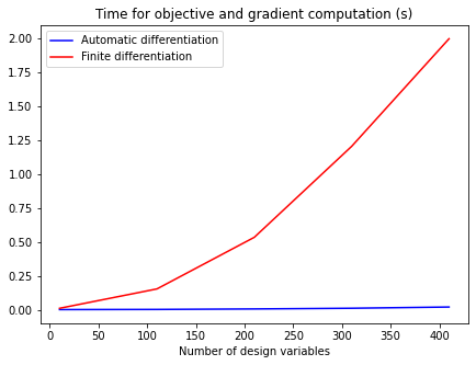
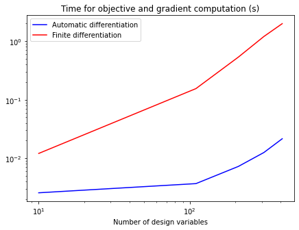
We now compare the computation time required to compute the gradient of the objective between PyTorch’s automatic differentiation and finite-difference approximation to the gradient which is what would be used if the gradient of the objective was not available (for example, in scipy.optimize).

The number of design variables are varied by considering a different discretization of wing to give a number of design variables that vary from \(10\) to \(500\). For finite differentiation, we consider a 2-step (a forward- or backward-step) method.

The results are ploted on both a linear scale and a log-log scale. It is evident that the automatic differentiation method is much faster, particularly when there are a large number of design variables. For \(400\) design variables, automatic differentiation is \(~100\times\) faster than finite differentiation. This is because the time to compute the gradient by automatic differentiation is effectively constant with respect to the number of design variables, assuming the cost of the objective doesn’t increase with the dimensionality. This assumption is violated in our case; however, the favorable scaling is still evident.

num_design_variables = torch.arange(10, 500, step=100)
num_trial = 10
t_finite_diff = torch.zeros((num_design_variables.numel(), num_trial))
t_auto_diff = torch.zeros((num_design_variables.numel(), num_trial))
for i,ndv in enumerate(num_design_variables):
    # setup model and optimization problem
    wing = Wing(Cl_target=0.5, num_discretize=ndv)
    optimizer = torchmdo.Optimizer(
        initial_design_variables=[torchmdo.DesignVariable(name="chords", lower=0.)],
        model=wing,
        objective=torchmdo.Maximize(name="span_efficiency_factor"),
        constraints=[],
    )
    x = optimizer.variables_tensor.detach()
    # run the trials for each gradient computation
    for trial in range(num_trial):
        # time the computation of the value and gradient by autograd
        optimizer.reset_state()
        t0 = time()
        optimizer.objective_fun(x)
        optimizer.objective_grad(x)
        t_auto_diff[i, trial] = time() - t0
        # time the finite difference gradient
        # for two-step forward finite difference this requires (1 + ndv) objective evaluations
        # so we will just evaluate it once and then multiply the time by this factor
        optimizer.reset_state()
        with torch.no_grad(): # ensure no overhead
            t0 = time()
            optimizer.objective_fun(x)
            t_finite_diff[i, trial] = (time() - t0)*(1 + ndv)
# plot
for plot_type in [plt.plot, plt.loglog]:
    plt.figure(figsize=(7,5))
    plot_type(num_design_variables, t_auto_diff.mean(dim=1), 'b', label="Automatic differentiation")
    plot_type(num_design_variables, t_finite_diff.mean(dim=1), 'r', label="Finite differentiation")
    plt.legend(loc=0)
    plt.title("Time for objective and gradient computation (s)")
    plt.xlabel("Number of design variables");